Regression Analysis

More pages in this category:

Choice Models - A Self Instructing Course

Iterative Proportional Fitting

Regression Analysis

Introduction

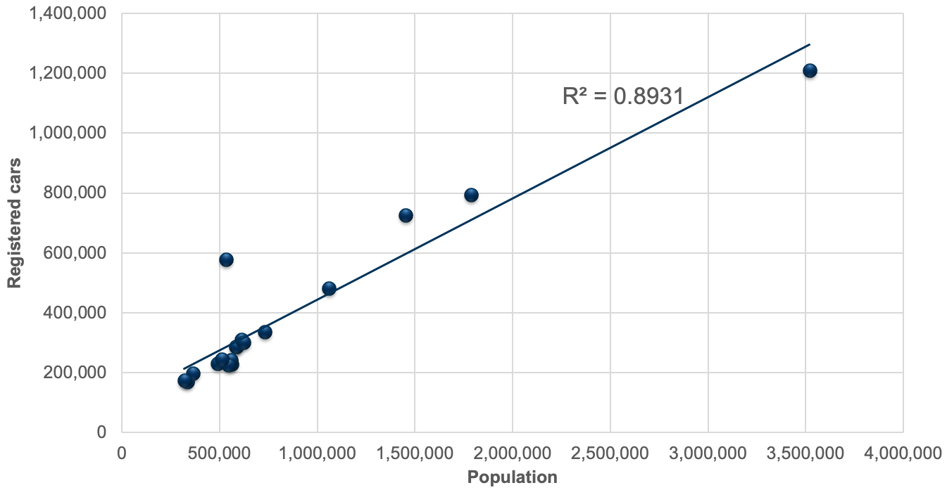
Regression analysis serves to explore the relationship between different variables, such as the number of cars registered in a city and the population of a city. This figure shows that there is -- not surprisingly -- a close relationship between the population in a city and the number of cars registered.

We write can write this relationship as

Read: The number of is a function of (short for population) plus the error term (epsilon). The figure above shows that population does not perfectly predict the number of registered cars (otherwise, all point would align on a perfect diagonal line). The error term captures this missing information, as well as measurement errors and suboptimal model specifications. By collecting more data, we could reduce the error term .

is the dependend variable (also called response or target), and serves as the independent variable (also called inputs, regressors, covariates, features) with which we try to explain the number of cars registered in the city.

Purpose of regression analysis

The goal of regression analysis is to:

• Accurately predict unseen cases.
• Understand which independent variables affect the dependent variableby which degree.
• Assess the quality of the available predictors and inferences.

It should be emphasized that regression analysis only detects correlation, not causation.

Notation

The function is commonly written as , where is the usual notation of the dependent variable. In the simplest form, two parameters need to be estimated with a statistical software:

Where

• is a constant
• a paremeter that defines the impact of population on the number of registered cars
• is the population in a given city

Parameter estimation

Using the statistical software R, the coefficients were estimated as:

Variable	Estimate	Std. Error	t value	Pr(>|t|)
(Intercept)	105752.3	1.082e+05	-1.752	0.099
Population	0.3378216	2.287e-01	11.562	3.52e-09

Multiple R-squared: 0.8931, Adjusted R-squared: 0.8864

This estimate can be used in our equation as:

This equation can be used to calculate the number of registered cars for another city. For example, a city with a population of 500,000 would be expected to have 274,663 registered cars.

R-squared (or R^2) is an indicator for the model performance. A value closer to 1 suggests that the model is able to represent the observed value very well. A smaller R^2 suggests that the model is missing important variables to explain the dependent variable.

This example shows a linear regression analysis, which is the simplest form of regression analyses. Linear regressions are almost never ''correct'', but a linear model often serves as a good and interpretable approximation to the unknown true function.

Transformation of variables

It is also possible to apply transformations of independent variables (or even the dependent variable). For example, a polinomial transformation improves the model fit slightly:

Variable	Estimate	Std. Error	t value	Pr(>|t|)
(Intercept)	104.6245	5.99e+04	0.00	0.099
Population	0.5518616	1.08e-01	5.10	0.00013
Population^2	-0.0000000589	2.88e-08	-2.04	0.05929

Multiple R-squared: 0.916, Adjusted R-squared: 0.905

Using the resulting equation

The number of registered cars for a city with a population of 500,000 would be 261,321.

The most common transformations in regression analysis include:

• Logarithmic transformation:
• Power transformation:
• Polynomial transformation:

Multiple regression

Multiple regression takes into account more than one variable. The number of registered cars in a city might not only depend on the population but also on other local factors (such as quality of transit, walkability, average income, unemployment rate, etc.). Here, population density was added as a proxy for transit quality and walkability:

Variable	Estimate	Std. Error	t value	Pr(>|t|)
(Intercept)	-34027.57	6.79e+04	-0.50	0.624
Population	0.2843189	3.50e-02	8.12	7.2e-07
PopulationDensity	70.91963	3.11e+01	2.28	0.038

Multiple R-squared: 0.921, Adjusted R-squared: 0.91

Using the resulting equation

The number of registered cars for a city with a population of 500,000 and a population density of 2000 people per squarekilometer would be 249,971.

Adding more independent variables tends to improve the estimation results, i.e. the R^2 value tends to get larger. However, adding variables should be done with care. Additional variables should only be accepted under the following conditions:

• The estimated parameter is significant. This is indicated by the value in column Pr(>t). If this value is 0.1, it suggests that there is a 10% probability that this parameter was random and does not represent a true relationship in the data. Obviously, this value should be as small as possible. As a rule of thumb, estimates with values greater than 0.1 should be rejected. Exceptions can be made if the value is close to 0.1, and the sign and size of the parameter are as expected and perform well in sensitivity analyses.
• The sign of the estimated parameter is as expected. In the example given above, the sign on the population parameter has to be positive. Otherwise, the model would predict fewer cars for larger cities. For density, one should expect a negative sign, as denser cities tend to have better transit systems and tend to be more walkable. If the sign is the opposite of what should be expected, the variable should be removed.
• The size of the estimated parameter is as expected. Often, this can only be detected through sensitivity analysis. In the example above, one should should take the population and populationDensity of an ''average'' city and adjust the values for population and populationDensity up and down (one at a time). If the parameters are reasonable, the resulting number of registered cars will be plausible.
• The independent variables shall not correlate with each other. If they do, so-called multicollinearity affects the estimation results. Commonly, multicollinearity leads to unexplainable estimated coefficients that result in nonsensical sensitivities.

If two models perform similarly well, but one uses more independent variables, the model with fewer independent variables is commonly preferred.

Variable interactions#

It is further possible to include interactions between two variables. One could hypothesize, for example, that higher densities only matter in cities with larger population. This effect can be represented by multiplying the two variables with each other.

Variable	Estimate	Std. Error	t value	Pr(>|t|)
(Intercept)	-71567.59	1.56e+05	-0.46	0.65
Population	0.351898	2.54e-01	1.39	0.19
PopulationDensity	81.14237	4.97e+01	1.63	0.13
Population PopulationDensity	-0.00001758771	6.54e-05	-0.27	0.79

Multiple R-squared: 0.921, Adjusted R-squared: 0.91

In this example, however, all estimated parameters did not reach a significance level of 0.1, and the estimation should be rejected.