Count Models

This page discusses why count models are necessary in certain applications, and discusses beginning details of the Poisson, negative binomial, and hurdle models.

Continuous versus count outcomes

Typical regression models are aimed at predicting the response of an outcome variable to a series of input variables . The result is a linear equation of a vector that describes the relationship between each element of and the outcome .

This regression framework assumes that is a continuous variable, meaning that it can take any numeric value within a particular range. The plot below shows the relationship between the average distance between home and workplace for workers in the household on the axis, and the household VMT on the axis, for households in smaller cities who responded to the 2017 NHTS. Both of these variables are continuous, meaning that a simple regression model is appropriate, though more information might need to be added to the model below to improve its fit and help explain outlying observations or control for heteroskedasticity.

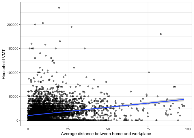
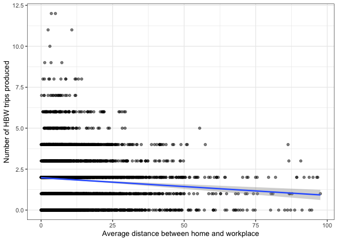
But consider the plot below, showing the same axis but with the number of home-based work trips produced by each household on the axis. Because the number of trips is discrete and not continuous, the plot looks kind of funny. But more importantly than this, we want a model that will predict a discrete number of vehicles as an outcome variable, and the blue regression line we estimated below will predict between 2 and 1 trips household; this isn't ideal.

Poisson Model

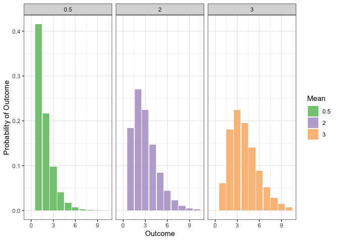
A better option would be to predict a probability that each household will produce a certain discrete number of trips. One way to do this is with a Poisson regression model. In this model, an analyst predicts the mean of a Poisson distribution with a regression equation (instead of a line). The Poisson distribution is:

where the probability of a discrete outcome is determined by the mean of the distribution. The plot below shows how as the mean increases, the probability of higher outcomes increases.

A Poisson regression model allows attributes of an observation to affect the value of the mean. So instead of in the linear regression, we now have , and gets put into the distribution equation above. In the model below, average work distance decreases the average number of trips, but more workers and more vehicles increases the average number.

	Linear	Poisson
(Intercept)	-0.106	-0.570***
	(-1.625)	(-13.865)
avg_workdist	-0.010***	-0.006***
	(-6.851)	(-7.070)
wrkcount	1.168***	0.665***
	(29.000)	(28.801)
hhvehcnt	0.147***	0.089***
	(5.626)	(5.925)
Num.Obs.	5533	5533
R2	0.185
R2 Adj.	0.185
AIC	19111.6	17871.7
BIC	19144.7	17898.1
Log.Lik.	-9550.813	-8931.830
F	419.097

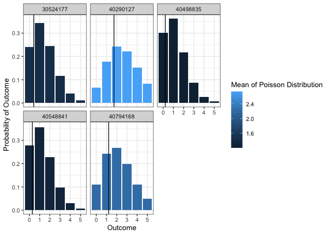
Of course, this is just an average. In a trip-based model, this average for each household might be sufficient. But you could also simulate a discrete choice for each person. The plot below shows the probability of a certain number of trips made by a sample of households, alongside what the predicted Poisson mean was. Households with a higher predicted mean have a higher probability of making more trips.

Negative Binomial Model

The Poisson model assumes that the mean and standard deviation of the distribution are the same. This can be a bad assumption, because it forces the distribution to spread out when the mean is higher. The negative binomial model relaxes this assumption, and might be useful in some contexts.

Hurdle Model

The Poisson and negative binomial models assume the same distribution across all outcomes; this might not be desirable if the number of zeros is high or low for some structural reason. For example, owning zero vehicles is very different from owning one or two. A hurdle model breaks the distribution into two different components:

• A binomial model determines the probability of choosing zero versus a positive number.
• A poisson or negative binomial model (with zero removed) determines the probability of a specific positive number, conditioned on the previous model.

References

1. UCLA Stats (opens new window)