Trend models in project-level traffic forecasting
# Objective
A linear trend model is a simple statistical technique to extrapolate upon historical traffic counts. Trend models can be used to forecast the inputs to a regional travel model, to forecast the inputs to a more complex statistical model of traffic volumes or to forecast directly traffic volumes from a time series of traffic count data.
# Background
A recently completed survey for NCHRP Report 765 found that linear trend models are widely used by state departments of transportation for project level forecasting purposes. A linear trend model can be readily accomplished with bivariate linear regression analysis, typically with traffic count as the dependent variable and time as the independent variable. Time is an integer number corresponding to the number of years from a reference year. A linear trend model has the form:
Tn = an+b
Where Tn is the forecasted traffic count, n is the year, and b is the forecasted traffic count in the reference year. The standard error of the forecast, S, may be taken as the 68% error range. The 50% error range may be computed from the standard error by this formula.
E50 = 0.6745S
Statistical software packages will also provide a t-score for the trend term, which will indicate whether the trend is sufficiently strong for forecasting purposes.
# Guidelines
Historic traffic counts should be plotted against time, to assure that there is a good trend in the data and that there are no anomalies. For consistency the reference year (e.g., 1991) should be held constant across all forecasts. It is possible for this reference year to be prior to the opening year for the road being studied, and thus it is possible for the constant b (y-intercept) to be a negative number. Choosing a recent base year aids the comparison of y-intercepts from linear regressions at different sites.
Both coefficients, a and b should be used in the forecast. The forecast should not pivot off the most recent traffic count. There should be a minimum of ten different years of historical traffic counts. The newest count should not be more than three years old. Forecasts should not extend farther into the future than historical data extends into the past. For example, a 20 year forecast should have historical data from at least 20 years ago.
The primary statistic for indicating the strength of the estimate is the t-score. The absolute value of the t-score of the trend term should not be less than 3.0, which indicates that the coefficient on the trend term is good to about one-half of a significant digit.
# Advice
Growth factor methods (i.e., models that assume a constant percent increase in traffic for each time period) should not be used, due to their inherently optimistic forecasts of traffic growth.
It is possible to forecast intersection turning movements by forecasting the volumes (in and out) on all legs of the intersection with trend models and then using an intersection refinement method (See Turning movement refinements).
Scenarios are difficult to introduce into trend forecasts, so scenarios are usually not formulated. If desired, “high growth” and “low growth” scenarios can be computed by adding or subtracting a fixed percentage from the yearly growth rate.
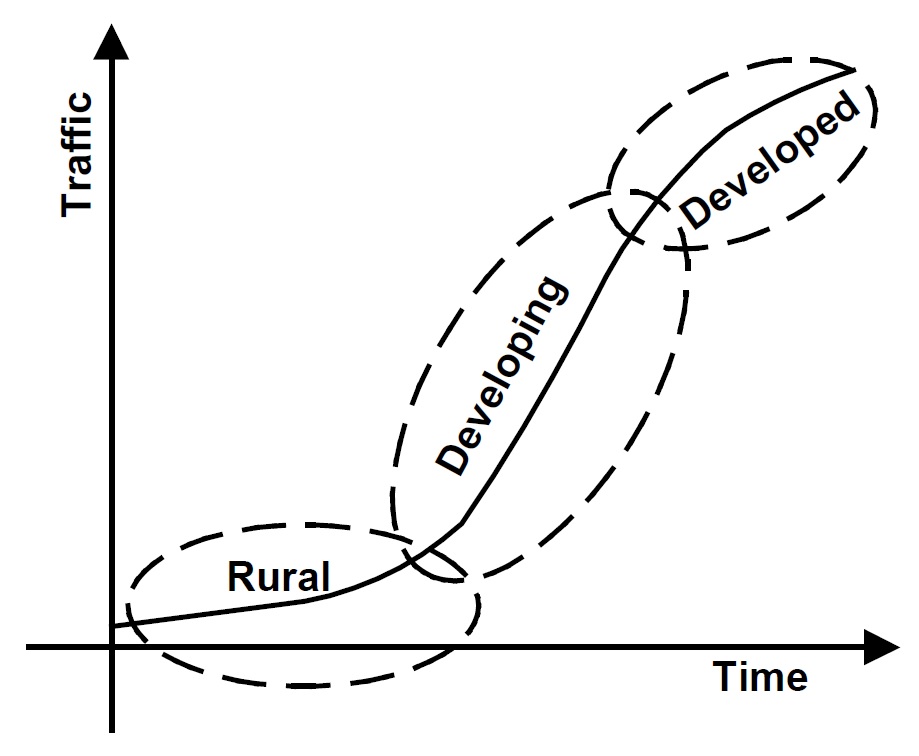
The analyst needs to be aware of the state of land use development near the highway segment when assessing how well a linear equation will forecast into into the distant future. Traffic growth could be accelerating or decelerating depending upon the degree to which land has been saturated. The figure below, originally published in the Guidebook on Statewide Travel Forecasting, illustrates how the rate of traffic growth can vary.

# Items to Report
- Regression statistics, including R<sup2, standard error of the estimate, and the t-score on the trend term.
- Forecasted traffic volume for the design year.
- The range associated with the 50% error in the forecast.
# References
NCHRP Report 765.
