Destination Choice Set Formation
This page is part of the Category [.
# Introduction
Choice set formation is a critical step in the specification, estimation, and application of discrete choice models. As noted by Thill (1992) (opens new window), the misspecification of choice sets can have adverse effects on parameter estimates and resultant computations of predicted choice probabilities. The accurate definition of the destination choice set has been an issue of much interest to the profession and a variety of approaches have been developed and adopted in research and practice. The problem is of acute significance in the context of destination choice modeling because the number of elemental alternatives can be very large. With many travel demand model systems comprising thousands of zones, destination choice sets can prove to be extremely large. On the one hand, methodological and computational advances allow the use of the universe of locations as the destination choice set. On the other hand, the use of universal set of destinations as the choice set may compromise the behavioral representativeness of destination choice models. The analyst needs to consider the pros and cons of alternative approaches carefully when defining destination choice sets.
A summary of approaches is presented in this page.
# Rule-based Approaches
Rule-based approaches are largely based on assumptions that the analyst makes about criteria that define the inclusion or exclusion of an elemental alternative in a destination choice set. This approach to location choice set formation has been used by Bowman et al (2015) (opens new window) in the context of location choice model estimation for the Puget Sound Regional Council SoundCast (opens new window) activity-based travel demand model.
When setting rules for destination choice set formation, specific criteria may be considered:
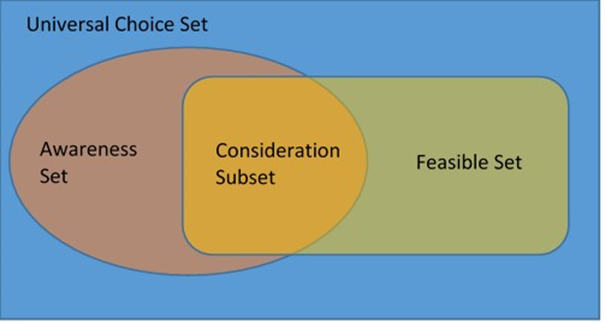
Feasibility: Based on information contained in observed choice data, the analyst may establish feasibility criteria for inclusion of an element in a choice set. For example, based on a cumulative trip length distribution for shopping trips in a travel survey data set, the analyst may specify a distance threshold beyond which shopping locations would be considered infeasible and therefore excluded from the ‘feasible’ choice set. For example, Bowman et al (2015) adopt a distance threshold equal to 125% of the longest trip distance (for a specific trip purpose) reported in the travel survey used for model estimation. While such feasibility criteria are often data-driven, they ignore heterogeneity in choice set formation and assume that a one-size-fits-all rule can be applied to the entire population. While a feasibility criterion may appear reasonable in the aggregate, it is unlikely to hold true in individual circumstances.
Awareness: As mentioned earlier, the universe of possible destinations can be very large. Individuals are not realistically able to consider and gather complete information on all possible destinations in the region. Given limited information gathering and processing capabilities of humans, and the possibility that individuals search until they are satisfied (satisficing rule), it is likely that individuals are aware of only a subset of alternatives as possible destinations and evaluate (in detail) only those alternatives that comprise the subset. Also, in many choice contexts, individuals may deliberately choose to narrow their search to a subset of alternatives, thus leading to the formation of an awareness set. It should be noted that awareness criteria can be combined with feasibility criteria to form a smaller subset of alternatives that constitute the intersection of these two sets of criteria. This smaller subset would then only include those alternatives that the individual considers feasible and is able to obtain full information to make an informed choice. In the absence of data about alternatives that individuals are aware of, it is difficult to establish robust awareness criteria for inclusion of alternatives in a choice set.
Figure 1. Depiction of Choice Sets
Trip Type – Land Use Compatibility: In most travel modeling contexts, it is possible to enhance feasibility criteria to consider the compatibility between trip type and land use characteristics. For example, one may choose to: exclude zones that have no jobs (employment) as possible work locations; exclude zones that have no student (enrollment) as possible school locations; exclude zones that have no retail employment as possible shopping locations; and exclude zones that have no housing stock as possible residential locations. All of these rules can help reduce the size of the consideration choice set in location choice modeling. The application of these compatibility rules is equivalent to using size variables in the utility equations to control the consideration/feasibility of zones. Thus, even if they are included in a choice set, zones that have a ‘zero’ size on a specific variable would be eliminated from consideration as a feasible destination for a specific trip type. This criterion may also consider the time-of-day at which a trip is being pursued; for example, if a shopping trip is being undertaken late at night, then only those destinations where establishments are open and operating at the time of the trip/activity (and known to the individual) would be included in the consideration choice set.
# Time-Space Prism Approaches
Time-space prisms represent activity spaces within which individuals may travel and pursue activities. The notion of a time-space prism is derived from the field of time geography (opens new window) Miller and Bridwell (2009) (opens new window) and has been used extensively in constructing activity-based travel demand model systems. The time-space prism constitutes a constrained action space that limits the range of destinations that an individual can visit. The time-space prism is often defined by boundaries or anchors that describe places where an individual must be present by a certain time (or within a specific narrow time window). These spatio-temporal bounds define a prism, with the size of the prism determined by the separation between the spatio-temporal boundaries and the speed of travel. Based on a knowledge of spatio-temporal constraints, the analyst can identify the feasible destination choice set as consisting of all possible locations that can be reached without violating a time-space prism constraint. The set of destinations that may be visited depends on the speed of travel; if the mode for a trip or tour is known a priori, then the speed of the mode can be used to determine prism size. If mode is determined subsequent to destination choice, then the set of reachable destinations may be identified based on the speed of the fastest available mode or a (weighted) average speed of all feasible modes. Time-space prism constraints can be further combined with feasibility and/or awareness criteria as well as land use availability criteria to identify a final subset of destinations that may be considered for a trip. Care must be exercised in the use of this approach to defining destination choice sets. Time-space prism constraints can be fuzzy and difficult to define, especially in the absence of specific data collected by survey samples about spatio-temporal constraints. For individuals who do not have anchor activities (such as work or school), the prism can be extremely large – resulting in a large set of possible destinations that may be reached without violating prism constraints. However, it is unlikely that individuals will consider such large choice sets when making location decisions.
Figure 2. Depiction of Time-Space Prism (Source: Miller and Bridwell, 2009)
# Sampling Approaches
The use of the multinomial logit (MNL) formulation for discrete models of destination choice makes it feasible to adopt sampling approaches without adversely affecting properties of parameter estimates. By virtue of the Independence of Irrelevant Alternatives (IIA) (opens new window) property, extreme value based discrete [ possess the desirable feature of accommodating sampling of alternatives without any deleterious effects. Considering that individuals are unlikely to consider thousands of alternatives when making location choices, it is appealing to adopt sampling approaches that may be more behaviorally defensible (from the standpoint that individuals can possible gather and process information only for a subset of alternatives when making location decisions). In sampling approaches, samples of 30, 50, or 100 locations are chosen from the universe of (feasible) choices – together with the chosen alternative. Multinomial logit models of destination choice are estimated on these sampled subsets of destination choices.
Two sampling approaches are quite commonly employed. These include random sampling and importance sampling. In random sampling approaches, the analyst draws a random sample of locations from the universe of (feasible) choices to constitute the consideration choice set. In this scheme, each and every alternative in the universe of (feasible) choices has an equal probability of being drawn into the consideration choice set.
In importance sampling approaches, the choice set composition method recognizes that some destinations are likely to be considered more highly (and thus considered more important or desirable) than others. An importance function is defined for each zone based on size and distance variables. Using Monte Carlo simulation (opens new window) procedures, a number of destinations are sampled with replacement from the importance probability distribution. Appropriate sampling correction factors need to be applied in estimation to retain desirable properties of the maximum likelihood estimator. A detailed description of the importance sampling function, the sampling correction factors, and the potential to combine importance sampling with sample explosion is available here (opens new window). Sample explosion involves replicating trip records with sampled choice sets for each exploded/replicated trip record. It has been found that sample explosion returns parameter estimates and standard errors equivalent to using a destination choice of size equal to the product of the number of replications per trip record and the number of sampled alternatives per record.
# Using the Universe of Location Alternatives
Methodological and computational advances now make it feasible to estimate discrete choice models with thousands of alternatives. In general, it is advisable to use the universe of destination choices when applying destination choice models in forecasting mode. For model estimation, sampling remains a popular approach to choice set formation, but the ability to use the universe of alternatives as the estimation choice set has proven increasingly appealing. Although the use of the universe of alternatives as the choice set for model estimation may be questioned from a behavioral decision-making perspective, it does eliminate pitfalls associated with sampling approaches. Sampling approaches involve the use of Monte Carlo drawing procedures, thus subjecting the formation of the choice set dependent on and susceptible to the choice set sampling process. In turn, model parameters and standard errors are also susceptible to the choice set sampling process. In order to eliminate the effects of sampling, it may be desirable to use the universe of alternatives to form the choice set. The gains from a statistical perspective should be weighed against the behavioral representativeness of such an approach when making decisions regarding the specification and estimation of destination choice models.
Theoretical behavioral basis for the use of the universe of alternatives together with psychological boundary terms and/or accessibility variables may be found in the work of Cascetta and Papola, 2001,[1] who show how the availability/perception of alternatives in the choice set can be reflected implicitly by terms in the systematic utility function. Psychological boundary terms and/or accessibility variables may play this role in destination choice models. Fotheringham, in particular, related his use of an accessibility term in his Competing Destinations model to a theory of choice set formation.[2]
# The Modifiable Areal Unit Problem (MAUP)
The Modifiable Areal Unit Problem (MAUP) (opens new window) arises due to the geographic aggregation of elemental location alternatives into zones or similar aggregate spatial units. Locations are often individual point or parcel locations (such as an individual home, building, office, or store), and yet choice alternatives in spatial location models are represented as zonal aggregations of such locations. The definition and delineation of traffic analysis zones (TAZ) affects the magnitudes and properties of model parameter estimates. The Modifiable Areal Unit Problem (MAUP) is thus a source of statistical bias that can significantly affect inference regarding the influence of various factors on destination choices (Fotheringham and Wong, 1991) (opens new window). The MAUP is an issue in destination choice modeling even though size terms used as explanatory variables in destination choice utility equations enter in log form, thus ensuring that choice probabilities change in direct proportion to the change in intensity of activities. Because of the MAUP, caution should be exercised in the application of destination choice models in forecasting mode. The zonal configuration used in model estimation should be retained in model application as well. A destination choice model estimated on one zonal configuration should not be applied to a vastly different zonal configuration. While very minor or modest deviations in zonal configuration may be acceptable in application mode, such deviations should be kept to a minimum. The choice set should therefore consist of traffic analysis zones (TAZ) that are defined with care, essentially eliminating or minimizing spatial autocorrelation problems through the definition of disaggregate homogeneous zones.
Within the mathematical formulation of the destination choice model, the implications of the MAUP on the size terms can be addressed from two perspectives: either the boundaries of the zones can be considered as a substantially artificial constructs of the model, or the boundaries of the zones can be considered as meaningful (if limited) expression of spatial auto-correlation. In the first case (zone boundaries are meaningless) then the individual activity opportunities within a zone should be considered no more similar to each other than to opportunities in other zones; this is achieved mathematically by fixing the coefficient on the size log term in the utility function exactly equal to 1.0. If, on the other hand, the zonal boundaries are meaningful, that implies that there is greater similarity among the individual activity opportunities within a zone than there is between those activities and others outside the zone. In this case, the coefficient on the size log term in the utility function should be constrained to take on a value between 0 and 1, analogous to a nested logit model for activities. A more detailed mathematical exposition for this is available here.
# Disaggregate Representation and Allocation of Activity Locations
With the adoption of increasingly disaggregate representation of space, the travel demand modeling profession is increasingly utilizing fine-grained units of geography to identify locations and destinations. For example, activity locations can be represented as points (on network links) or individual parcels. More recently, activity based models have been adopting the use of microanalysis zones (MAZ) (opens new window) as a unit of geography to represent destination and location choices at a fine-grained spatial resolution and better capture transit access and egress legs. Bowman et al (2015) describe location choice model specification and estimation using parcel level geography for the Puget Sound Regional Council activity-based travel demand model called SoundCast.
Multi-step procedures may be adopted to spatially allocate households, persons, or trip ends to individual parcels, MAZs, or point locations. After allocating locations to regular traffic analysis zones (TAZ) or similar aggregate geographic units (census tract or block group, for example), additional procedures may be implemented to further disaggregate locations to finer spatial scale. Such spatial disaggregation may be accomplished based on distribution of population or employment across the smaller geographical units that comprise the zone, distribution of street network density, or other measures of land use appropriate to sub-allocation of activity locations. More sophisticated procedures in which synthetic populations generated at an aggregate geographic scale are further spatially sub-allocated to the parcel level have also been developed (Zhu and Ferreira, 2014) (opens new window). Such procedures employ iterative processes at multiple geographic scales to allocate households to individual parcels while controlling for known parcel capacity constraints and estimated conditional distributions of household attributes by building type.
# References
Content Charrette: Destination Choice Models
Bowman, J., M. Bradley, and S. Childress (2015) Location Choice Model Estimation. SoundCast: Activity-Based Travel Forecasting Model. Puget Sound Regional Council, Seattle, WA. Available at: 1 (opens new window)
Fotheringham, A.S. and D.W.S. Wong (1991) The Modifiable Areal Unit Problem in Multivariate Statistical Analysis. Environment and Planning A, 23(7), pp. 1025-1044. Available at: 2 (opens new window)
MTC and PB, Inc. (2013) Travel Model Two: Initial Representation of Space. Metropolitan Transportation Commission with Parsons Brinckerhoff, Inc., San Francisco, CA. Available at: 3 (opens new window)
Miller, H. and S.A. Bridwell (2009) A Field-Based Theory for Time Geography. Annals of the Association of American Geographers 99(1), pp. 49-75. Available at: 4 (opens new window)
Thill, J-C. (1992) Choice Set Formation for Destination Choice Modeling. Progress in Human Geography 16(3), pp. 361-382. Available at: 5 (opens new window)
Zheng, J. and J.Y. Guo (2008) Destination Choice Model Incorporating Choice Set Formation. Compendium of Papers of the 87th Annual Meeting of the Transportation Research Board, Washington, D.C.
Zhu, Y. and J. Ferreira Jr (2014) Synthetic Population Generation at Disaggregated Spatial Scales for Land Use and Transportation Microsimulation. Transportation Research Record: Journal of the Transportation Research Board 2429, pp. 168-177. Available at: 6 (opens new window)
Cascetta, E. and A. Papola. 2001. Random utility models with implicit availability/perception of choice alternatives for the simulation of travel demand. Transportation Research Part C: Emerging Technologies, Vol. 9, No. 4, pp. 249–263. https://doi.org/10.1016/S0968-090X(00)00036-X (opens new window) ↩︎
Fotheringham, A. S. Consumer Store Choice and Choice Set Definition. Marketing Science, Vol. 7, 1988, pp. 299–310. ↩︎